Overview of the Problem

The textbook presents the following scenario:

“Imagine tossing a ball vertically at an initial speed of 20 m/s. Assume the acceleration due to gravity is 10 m/s². How long will it take for the ball to return to the ground, disregarding air resistance?” — Gibiliseo (2007, p. 26)

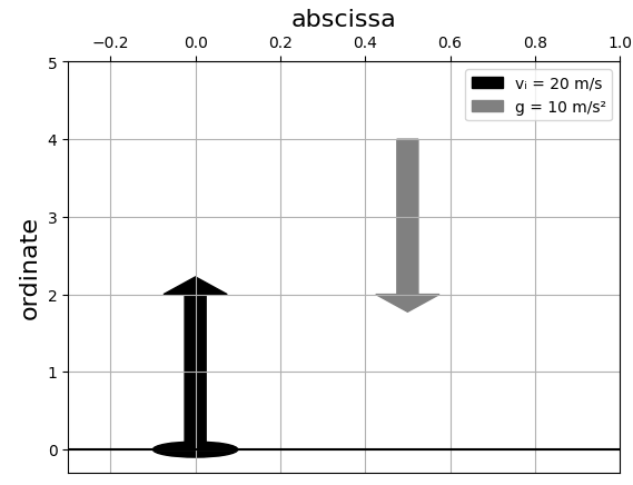
Before diving into the solution, I wanted to visualize the scenario. Below is an illustration of my conceptualization:

For this discussion, I will focus on the kinematic equations that define the ball's velocity and displacement as functions of time.

Formulating the Solution

The connection between displacement, velocity, and acceleration is captured in the following equation:

In this formula, a(t) represents acceleration, v(t) denotes the velocity function, h(t) corresponds to displacement, and t is an independent variable symbolizing time. Given an acceleration function, in this case, a(t) = -10 m/s², we can derive the velocity and displacement functions using integrals.

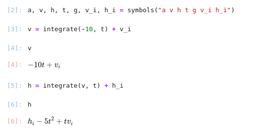
Python and the SymPy Live Shell (n.d.) make this process straightforward, as illustrated in the following image:

Upon manually solving this problem, I obtained the displacement function -5t² + v_it + h_0, which aligns with the solution generated by SymPy Live Shell. The question remains: “[h]ow long will it take for the ball to return to the ground, neglecting air resistance?”

To answer, I applied the general solution for quadratic equations, leveraging the initial velocity v_i = 20 m/s. For simplicity, units will be omitted until the final solution.

Notably, the problem specifies that the height h_0 is at the origin (0, 0) on the Cartesian plane. This allows us to simplify the quadratic equation, resulting in:

I implemented and solved for t_1 and t_2 using Python as follows:

>>> import math

>>> t_1 = lambda a, v_i: (-v_i + math.sqrt(v_i**2)) / (2 * a)

>>> t_2 = lambda a, v_i: (-v_i - math.sqrt(v_i**2)) / (2 * a)

>>> t_1(-5, 20)

-0.0

>>> t_2(-5, 20)

4.0

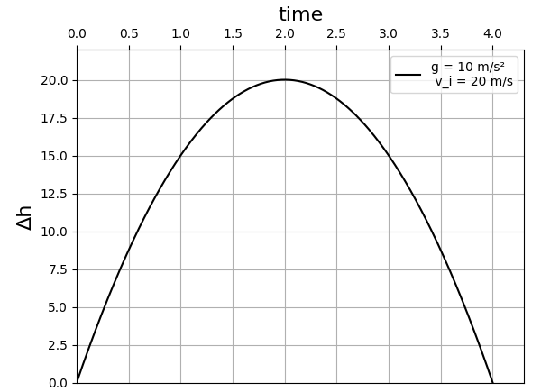
Thus, the solutions for t are 0 seconds and 4 seconds. Logically, the duration it takes for the ball to return to the ground is approximately four seconds, occurring after it reaches its peak height. The following graph illustrates the height displacement function, providing a visual representation of the solution:

Python in Physics Problem Solving

Through this article, I have explored how Python can be a valuable tool in addressing physics-related problems. While I believe that Python enhances the process of solving applied math challenges, it should not completely replace the traditional methods, which, although labor-intensive, are critical for understanding.

Acknowledgments

I would like to express my gratitude to Amit Saha for his book "Doing Math with Python" (Saha 2015), which served as a valuable reference in writing this article and developing Python code.

Appendix

A. Code for Figure 1

import matplotlib.pyplot as plt

plt.figure()

ax = plt.gca()

plt.rcParams['xtick.bottom'] = plt.rcParams['xtick.labelbottom'] = False

plt.rcParams['xtick.top'] = plt.rcParams['xtick.labeltop'] = True

plt.axhline(color="black")

plt.arrow(0, 0, 0, 2, label="v_i = 20 m/s", width=0.05, color="black")

plt.arrow(0.5, 4, 0, -2, label="g = 10 m/s²", width=0.05, color="grey")

circle = plt.Circle((0, 0), radius=0.1, color="black")

ax.add_patch(circle)

plt.legend()

plt.grid()

plt.title("Abscissa", fontsize=16)

plt.ylabel("Ordinate", fontsize=16)

plt.xlim(-0.3, 1)

plt.ylim(-0.3, 5)

plt.show()

B. Code for Figure 3

import math

import matplotlib.pyplot as plt

import numpy as np

plt.figure()

plt.rcParams['xtick.bottom'] = plt.rcParams['xtick.labelbottom'] = False

plt.rcParams['xtick.top'] = plt.rcParams['xtick.labeltop'] = True

h = lambda t: -5*t**2 + 20*t

T = np.arange(0, 5, 0.01)

plt.plot(T, [h(t) for t in T], color="black", label="g = 10 m/s² n v_i = 20 m/s")

plt.legend()

plt.grid()

plt.title("Time", fontsize=16)

plt.ylabel("Height (h)", fontsize=16)

plt.xlim(0, 4.3)

plt.ylim(0, 22)

plt.show()

References

Gibiliseo, S. (2007). Advanced Physics Demystified [Paperback]. McGraw-Hill Education.

Saha, A. (2015). Doing Math with Python: Use Programming to Explore Algebra, Statistics, Calculus, and More! No Starch Press.

The first video, "Python Physics: Motion of a Ping Pong Ball WITH Air Drag," explores the effects of air drag on projectile motion, providing insights relevant to our discussion.

The second video, "Python Physics Lesson 5: Projectile Motion with Air Resistance," covers key concepts in projectile motion, enhancing understanding of these physics principles.