Chapter 1: Understanding Temporal Analysis

Temporal analysis is intrinsically linked to the aspect of time in trading. In technical analysis, our primary focus often revolves around price levels and their deviations from the norm. This article aims to clarify a straightforward approach that utilizes both time and extreme values derived from technical indicators, assessing whether they yield reliable signals. We will develop the indicator, construct the strategy, and subsequently evaluate its effectiveness.

I have recently published a new book following the success of my previous work. It showcases advanced trend-following indicators and strategies, along with a dedicated GitHub page for ongoing code updates. The book features original colors, optimized for printing costs. If this piques your interest, feel free to check the Amazon link below, or contact me via LinkedIn for a PDF version.

Book Resource:

Trend Following Strategies in Python: How to Use Indicators to Follow the Trend.

Chapter 2: The Trend Intensity Index

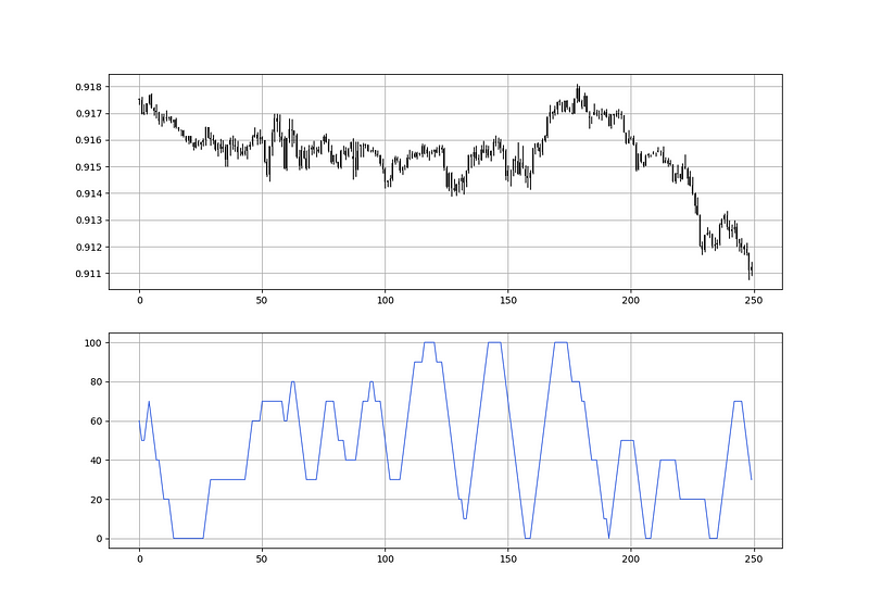
The Trend Intensity Index (TII) serves as a gauge for trend strength. This relatively simple metric is derived from a 10-period moving average and price variations around it. We will proceed with a step-by-step construction of the indicator:

1. Define a lookback period of 10 and compute the moving average for the market price.

lookback = 10

Defining the Primal Manipulation Functions

def adder(Data, times):

for i in range(1, times + 1):

new = np.zeros((len(Data), 1), dtype=float)

Data = np.append(Data, new, axis=1)

return Data

def deleter(Data, index, times):

for i in range(1, times + 1):

Data = np.delete(Data, index, axis=1)

return Data

def jump(Data, jump):

Data = Data[jump:,]

return Data

Defining the Moving Average Function

def ma(Data, lookback, close, where):

Data = adder(Data, 1)

for i in range(len(Data)):

try:

Data[i, where] = (Data[i - lookback + 1:i + 1, close].mean())

except IndexError:

pass

Data = jump(Data, lookback)

return Data

Next, we will calculate the deviations of the market price from the moving average, filling two columns based on whether the current market price is above or below its 10-period moving average.

for i in range(len(my_data)):

if my_data[i, what] > my_data[i, where]:

my_data[i, where + 1] = my_data[i, what] - my_data[i, where]

if my_data[i, what] < my_data[i, where]:

my_data[i, where + 2] = my_data[i, where] - my_data[i, what]

We will then count the instances where the market was above or below its 10-period moving average:

for i in range(len(Data)):

Data[i, where + 3] = np.count_nonzero(Data[i - lookback + 1:i + 1, where + 1])

for i in range(len(Data)):

Data[i, where + 4] = np.count_nonzero(Data[i - lookback + 1:i + 1, where + 2])

Finally, we can compute the Trend Intensity Index using the following formula:

for i in range(len(Data)):

Data[i, where + 5] = ((Data[i, where + 3]) / (Data[i, where + 3] + Data[i, where + 4])) * 100

EURUSD with the 10-Period Trend Intensity Index

The complete function for calculating the trend intensity index is as follows:

def trend_intensity_index(data, lookback, close, where):

data = ma(data, lookback, close, where)

data = adder(data, 5)

# Deviations

for i in range(len(data)):

if data[i, close] > data[i, where]:

data[i, where + 1] = data[i, close] - data[i, where]

if data[i, close] < data[i, where]:

data[i, where + 2] = data[i, where] - data[i, close]

# Trend Intensity Index

for i in range(len(data)):

data[i, where + 3] = np.count_nonzero(data[i - lookback + 1:i + 1, where + 1])

for i in range(len(data)):

data[i, where + 4] = np.count_nonzero(data[i - lookback + 1:i + 1, where + 2])

for i in range(len(data)):

data[i, where + 5] = ((data[i, where + 3]) / (data[i, where + 3] + data[i, where + 4])) * 100

data = deleter(data, where, 5)

return data

Chapter 3: The Duration Strategy

The structure of the Trend Intensity Index reveals that:

• An oversold reading near 0 suggests a diminishing bearish momentum, indicating a potential upward correction or reversal.
• An overbought reading at 100 implies a waning bullish momentum, hinting at a possible downward correction or reversal.

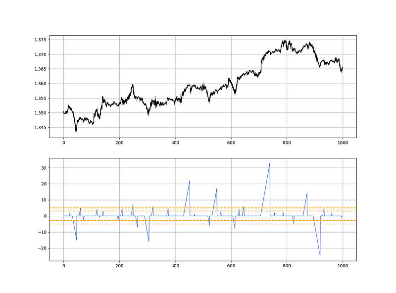
However, trading is rarely that straightforward. Our goal with temporal analysis is to determine the average duration the indicator spends in these extremes, combining both time and extremity to generate a signal. Below, a chart illustrates this more explicitly.

The above chart depicts the EURUSD alongside the number of periods the 3-period Trend Intensity Index has occupied the extreme zone. A reading of -3 indicates that the index remained at the zero level for three time periods. To calculate this Duration, follow the steps below:

1. Define the lookback period:

lookback = 3

2. Calculate the TII on the OHLC array (composed of four columns).
3. Add additional columns for further calculations.
4. Set the barriers for oversold and overbought zones:

upper_barrier = 3

lower_barrier = -3

Calculating the Extreme Duration

def extreme_duration(Data, indicator, upper_barrier, lower_barrier, where_upward_extreme, where_downward_extreme):

# Time Spent Overbought

for i in range(len(Data)):

if Data[i, indicator] == upper_barrier:

Data[i, where_upward_extreme] = Data[i - 1, where_upward_extreme] + 1

else:

Data[i, where_upward_extreme] = 0

# Time Spent Oversold

for i in range(len(Data)):

if Data[i, indicator] == lower_barrier:

Data[i, where_downward_extreme] = Data[i - 1, where_downward_extreme] + 1

else:

Data[i, where_downward_extreme] = 0

Data[:, where_downward_extreme] = -1 * Data[:, where_downward_extreme]

return Data

my_data = adder(my_data, 10)

my_data = extreme_duration(my_data, 4, 100, 0, 7, 6)

my_data[:, 8] = my_data[:, 6] + my_data[:, 7]

When the extreme duration enters the range between -3/-5 or 3/5, it suggests a market reaction is likely.

def signal(Data, what, buy, sell):

Data = adder(Data, 10)

for i in range(len(Data)):

if Data[i, what] <= -3 and all(Data[i - j, buy] == 0 for j in range(1, 5)):

Data[i, buy] = 1

elif Data[i, what] >= 3 and all(Data[i - j, sell] == 0 for j in range(1, 5)):

Data[i, sell] = -1

return Data

A considerable amount of optimization can be applied to this promising technique, especially since mere value readings have become insufficient. Understanding the temporal aspect is crucial for grasping how the underlying asset reacts.

If you are interested in learning about more technical indicators and strategies, my book may offer valuable insights.

Book Resource:

The Book of Trading Strategies

Chapter 4: Evaluating the Signals

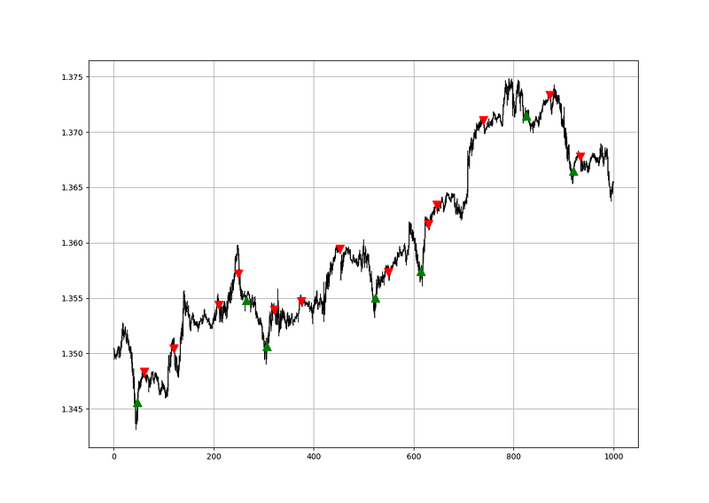
After generating signals, we can identify when the algorithm would have executed buy and sell orders. This simulation allows us to assess how the strategy would have performed under our specified conditions.

Calculating the returns and analyzing performance metrics will reveal insights into our trading effectiveness. For instance, our hit ratio stands at 54%, suggesting that out of 100 trades, approximately 54 would be profitable, excluding transaction costs. This indicates that the strategy, applied to hourly data for EURUSD since 2011 (approximately 932 trades), lacks significant predictive power. Future analysis should include other currency pairs and assets for a comprehensive assessment.

If you're keen on receiving more articles related to trading strategies, consider subscribing to my DAILY Newsletter, which includes a mix of Medium articles, additional trading strategies, coding tutorials, and free PDF copies of my first book. You can expect 5–7 articles weekly with a paid subscription and 1–2 articles with a free plan.

Newsletter Resource:

All About Trading!

Sharing Trading Strategies, Knowledge, and Technical Tools in Detail.

Remember, always conduct back-tests. It's crucial to approach trading with skepticism; what works for one trader may not work for another. I advocate for self-discovery, emphasizing the importance of grasping the underlying ideas, functions, and conditions of a strategy before refining it further.

Chapter 5: Final Thoughts

I have recently launched an NFT collection aimed at supporting various humanitarian and medical initiatives. The Society of Light is a limited collection of NFTs, with a portion of sales directly benefiting charitable causes linked to the avatars. Here are some key benefits of purchasing these NFTs:

• High-Potential Gains: The remaining sales proceeds focus on marketing and promoting The Society of Light, maximizing their value in the secondary market. Trading in this market also means a portion of royalties will be donated to the same charity.
• Art Collection and Portfolio Diversification: Owning avatars that symbolize good deeds is incredibly rewarding. Investing can extend beyond personal gain; it can also contribute positively to society.
• Flexible Donations to Preferred Causes: This allows for a personalized approach to supporting different charities.
• Free PDF Copy of My Book: Buyers of any NFT will receive a complimentary PDF copy of my latest book.